
A crypto backtest Sharpe ratio compares average return above a stated reference with the variability of that return series. It does not prove profit, predict a future result, or describe every kind of risk. Before comparing two scores, record the return interval, reference return, cost boundary, annualization method, sample dates, and treatment of open positions. Without those inputs, a precise-looking ratio may be comparing different questions.
What a crypto backtest Sharpe ratio measures
The common historical form can be summarized as:
Sharpe ratio = average differential return ÷ standard deviation of differential return
Differential return means the strategy return minus a stated reference return for the same interval. The reference might be a cash or risk-free rate, but the choice and data source must be documented rather than assumed.
In his primary 1994 article, William F. Sharpe explains the ratio as a reward-to-variability measure and distinguishes historical calculation from expectations about the future. He also notes that mean and variance cannot capture every relevant difference between return distributions. That limitation matters when a crypto backtest has concentrated losses, open exposure, or unusual market conditions.
The return interval is part of the result
A ratio built from daily returns and one built from weekly returns do not have the same raw scale. Sampling changes both the average and the standard deviation. If a platform annualizes the result, the annualization convention becomes another required input.
Write down whether the calculation uses trade returns, hourly returns, daily returns, or another series. Then confirm that the reference return uses the same interval. Do not compare two displayed ratios until the interval and annualization method match.
Same average return, different variability
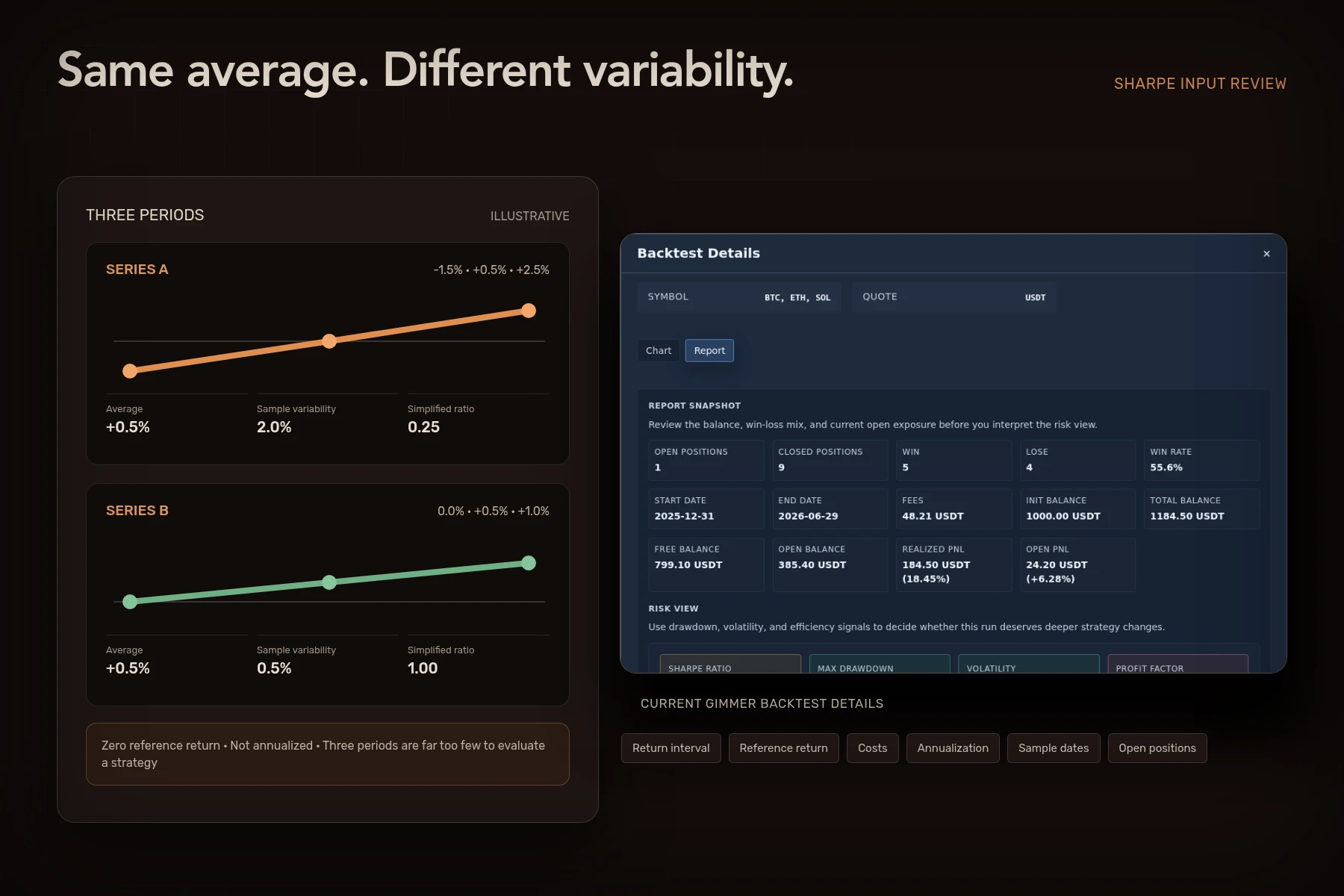
Consider two deliberately small, illustrative three-period series. Both have an arithmetic average return of 0.5% per period, and both assume a zero reference return:
| Input | Series A | Series B |
|---|---|---|
| Periodic returns | -1.5%, +0.5%, +2.5% | 0.0%, +0.5%, +1.0% |
| Arithmetic average | +0.5% | +0.5% |
| Sample standard deviation | 2.0% | 0.5% |
| Simplified, nonannualized ratio | 0.25 | 1.00 |
The second series has the higher simplified ratio because the same arithmetic average sits over a smaller denominator. These figures are not Gimmer results, market data, or a recommendation. Three observations are far too few to assess a strategy. The example only shows why the return path and calculation method matter.
Audit six inputs behind the score
- Return series: Record whether the input is based on trades, candles, daily equity, realized balance, or another defined series.
- Reference return: Name the comparator, its source, and how it was aligned to each interval.
- Cost boundary: State which fees and execution assumptions are already reflected. Use the backtest cost checklist to keep omitted costs visible.
- Variability convention: Record the standard-deviation convention and how missing or zero-return intervals are handled.
- Annualization: If the score is annualized, record the factor and confirm that the sampling interval supports it.
- Exposure treatment: State whether the series includes open PnL and how the final open position is valued.
If one input is unavailable, label the comparison incomplete. Do not infer the missing method from the number of decimal places.
Read Sharpe ratio beside drawdown and positions
Standard deviation treats movements around the average as variability. It does not tell you when the deepest loss occurred, how long recovery took, whether one position dominated the result, or whether an open loss remains unsettled.
Gimmer’s current guide to reading Backtest Details shows Sharpe Ratio inside Risk View alongside Max Drawdown, Volatility, Profit Factor, and the drawdown path. The same workflow keeps Report Snapshot and the Position journal in view. Use those sections together. A higher ratio does not override a loss path or trade record that you have not inspected.
Check the data and search process
A clean calculation can still summarize weak evidence. Missing candles, inconsistent timestamps, repeated parameter search, and selection from many discarded trials can all change the series that reaches the formula.
Start with the crypto backtest data checklist. Then record how many variations were tried using the overfitting trial log. Finally, challenge the locked revision with the out-of-sample testing workflow. None of these steps makes a historical score predictive, but each one makes its evidence boundary clearer.
Compare like with like
Use a Sharpe ratio to compare two historical runs only after these fields match or their differences are explicitly understood:
- market and quote currency;
- start and end dates;
- return interval and time zone;
- reference return and source;
- included costs and open-position treatment;
- annualization and standard-deviation method.
Even a fair historical comparison is not a forecast. It is a controlled way to ask why one tested path looked different from another.
Frequently asked questions
What is a good Sharpe ratio for a crypto backtest?
There is no universal threshold that makes a crypto strategy good or ready for live use. The value depends on the return series, reference, costs, interval, annualization, sample, and market conditions. Use it as one comparison input after the calculation boundary is known.
Can two platforms show different Sharpe ratios for the same strategy?
Yes. Different return intervals, reference returns, annualization factors, cost treatment, missing-data rules, and open-position valuation can produce different scores. Compare the methods before comparing the values.
Does a higher historical Sharpe ratio mean lower future risk?
No. It describes one historical return series under stated assumptions. It does not capture every risk, and it does not establish how future prices, liquidity, execution, or operations will behave.
Turn the score into a reproducible review
A Sharpe ratio is most useful when another reviewer can reconstruct what went into it. The score becomes less useful when the inputs disappear behind a ranking.
For the next historical run, open Gimmer’s Running Backtest guide and record the return interval, reference return, included costs, annualization method, sample dates, and open-position treatment beside the ratio. Keep drawdown and the position record open before you compare candidates, and treat every result as evidence about tested history rather than a promise about future trading.